Introduction

One of the great features of LAMMPS is that it can run on single processors or in parallel using message-passing techniques and a spatial-decomposition of the simulation domain. As it’s named acronym implies, Large-scale Atomic/Molecular Massively Parallel Simulator is well suited for parallelization in the cloud, and this article will review ways to optimize those simulations. This can work equally well for Molecular Dynamics and Materials Sciences simulations.

Background/Problem Statement (Boundary 3 - x, y, z)

If you were to take one of the example input files from the LAMMPS installation directory, you can run the simulations in a few seconds or minutes on a local or cloud machine. The challenge comes as you add complications to the simulation. Like a wristwatch, the expectation of telling time is pretty reasonable. As you add features or “complications” like perpetual date calendar, day of the week, lunar phases etc., to the timepiece, the difficulty to pack those complications into a portable wearable device becomes much more difficult. Adding multi-elemental compounds, varying energy levels, temperature phases or expanding the volumetric space within which the simulation occurs; can dramatically change the computational requirements. This also quickly goes beyond the reasonable potential of a single processor, local machine. The next challenge to overcome is how to assemble the environment that is suitable and optimizable for parallel computing in a cloud environment.

Solution (Breaking Out of the Box)

Taking to the cloud may be a bit overwhelming as the major cloud providers offer hundreds of services that are not woven together into a cohesive unit. CloudyCluster enables Parallel Computation aka High Performance Computing (HPC) enables researchers, investigators, engineers and others to take years of computation and complete them in hours by parallelizing and batching their workloads. The platform handles all of the security, networking and provisioning of computation needs, based on your job’s needs. Additionally, CloudyCluster spins up an image with dozens of open source scientific and research software packages ready to go. This simulation took a variety of samples and ran them in different MPI configurations of nodes and task divisions. CloudyCluster’s meta-scheduler CCQ handles the job transport from command line, to a database to queue the jobs, provides status and communicates issues with the jobs via CCQStat.

Simulations

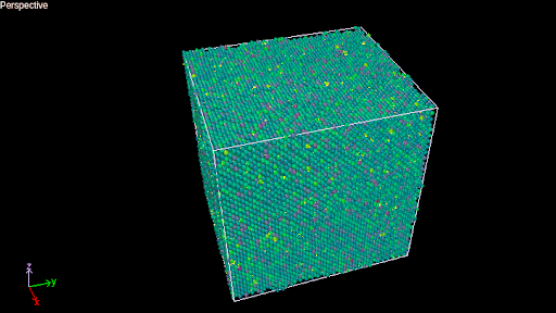
Using the calc_fcc.in input file, the material source of Al from , a simple single node MPI script took only seconds to process the output files, which can then be rendered in a visualization tool of choice. When that same input file is edited to enlarge the volume of the simulation space, from 1 1 1 to 1000 1000 1000, the single cpu local machine crashes but the CloudyCluster environment can scale with the needs of the job. The expanded simulation took under 5 minutes from submission to completion as 4 OrangeFS parallel nodes handled the file system duties, and in this case Slurm acted as the scheduler, spinning up 8 compute-group nodes handling 4 tasks per node. Using the OpenM environment variable ‘export OMP_NUM_THREADS=4’ to run the computations. When the simulation was completed, CCQ cleaned up the database entries, terminated the scheduler functions and tore down the compute group, scaling back the cluster enviroment to a standby ready state.

Post Processing Visualization

Sandia Labs has a list of recommended tools that you can use to view the results of the jobs. For the animation still shown above, PyMol was used to process and manipulate the output.

Next Steps

To give CloudyCluster a “spin” login to your GCP account and click the Marketplace link here. You can have a trial of CloudyCluster to get comfortable with what it can do for your research.

If you want to talk through the process, reach out to support@cloudycluster.com and a member of the team will get in touch with you.

Citings:

1. Input File: Mark A. Tschopp from his tutorial.
2. Sandia National Laboratory: LAMMPS
3. The PyMOL Molecular Graphics System, Version 2.0 Schrödinger, LLC. PyMol Website